Animal rescue incidents analysis
#Animal rescue incidents attended by the London Fire Brigade
The London Fire Brigade attends a range of non-fire incidents (which we call ‘special services’). These ‘special services’ include assistance to animals that may be trapped or in distress. The data is provided from January 2009 and is updated monthly. A range of information is supplied for each incident including some location information (postcode, borough, ward), as well as the data/time of the incidents. We do not routinely record data about animal deaths or injuries.
Please note that any cost included is a notional cost calculated based on the length of time rounded up to the nearest hour spent by Pump, Aerial and FRU appliances at the incident and charged at the current Brigade hourly rate.
url <- "https://data.london.gov.uk/download/animal-rescue-incidents-attended-by-lfb/f43b485e-fb35-419c-aa7a-fa75676e5835/Animal%20Rescue%20incidents%20attended%20by%20LFB%20from%20Jan%202009.csv"


animal_rescue <- read_csv(url,
                          locale = locale(encoding = "CP1252")) %>%
  janitor::clean_names()


glimpse(animal_rescue)
## Rows: 8,751
## Columns: 31
## $ incident_number <chr> "139091", "275091", "2075091", "2872091"…
## $ date_time_of_call <chr> "01/01/2009 03:01", "01/01/2009 08:51", …
## $ cal_year <dbl> 2009, 2009, 2009, 2009, 2009, 2009, 2009…
## $ fin_year <chr> "2008/09", "2008/09", "2008/09", "2008/0…
## $ type_of_incident <chr> "Special Service", "Special Service", "S…
## $ pump_count <chr> "1", "1", "1", "1", "1", "1", "1", "1", …
## $ pump_hours_total <chr> "2", "1", "1", "1", "1", "1", "1", "1", …
## $ hourly_notional_cost <dbl> 255, 255, 255, 255, 255, 255, 255, 255, …
## $ incident_notional_cost <chr> "510", "255", "255", "255", "255", "255"…
## $ final_description <chr> "Redacted", "Redacted", "Redacted", "Red…
## $ animal_group_parent <chr> "Dog", "Fox", "Dog", "Horse", "Rabbit", …
## $ originof_call <chr> "Person (land line)", "Person (land line…
## $ property_type <chr> "House - single occupancy", "Railings", …
## $ property_category <chr> "Dwelling", "Outdoor Structure", "Outdoo…
## $ special_service_type_category <chr> "Other animal assistance", "Other animal…
## $ special_service_type <chr> "Animal assistance involving livestock -…
## $ ward_code <chr> "E05011467", "E05000169", "E05000558", "…
## $ ward <chr> "Crystal Palace & Upper Norwood", "Woods…
## $ borough_code <chr> "E09000008", "E09000008", "E09000029", "…
## $ borough <chr> "Croydon", "Croydon", "Sutton", "Hilling…
## $ stn_ground_name <chr> "Norbury", "Woodside", "Wallington", "Ru…
## $ uprn <chr> "NULL", "NULL", "NULL", "1.00E+11", "NUL…
## $ street <chr> "Waddington Way", "Grasmere Road", "Mill…
## $ usrn <chr> "20500146", "NULL", "NULL", "21401484", …
## $ postcode_district <chr> "SE19", "SE25", "SM5", "UB9", "RM3", "RM…
## $ easting_m <chr> "NULL", "534785", "528041", "504689", "N…
## $ northing_m <chr> "NULL", "167546", "164923", "190685", "N…
## $ easting_rounded <dbl> 532350, 534750, 528050, 504650, 554650, …
## $ northing_rounded <dbl> 170050, 167550, 164950, 190650, 192350, …
## $ latitude <chr> "NULL", "51.39095371", "51.36894086", "5…
## $ longitude <chr> "NULL", "-0.064166887", "-0.161985191", …One of the more useful things one can do with any data set is quick counts, namely to see how many observations fall within one category. For instance, if we wanted to count the number of incidents by year, we would either use group_by()... summarise() or, simply count()
animal_rescue %>%
  dplyr::group_by(cal_year) %>%
  summarise(count=n())
## # A tibble: 14 × 2
## cal_year count
## <dbl> <int>
## 1 2009 568
## 2 2010 611
## 3 2011 620
## 4 2012 603
## 5 2013 585
## 6 2014 583
## 7 2015 540
## 8 2016 604
## 9 2017 539
## 10 2018 610
## 11 2019 604
## 12 2020 758
## 13 2021 885
## 14 2022 641animal_rescue %>%
count(cal_year, name="count")## # A tibble: 14 × 2
## cal_year count
## <dbl> <int>
## 1 2009 568
## 2 2010 611
## 3 2011 620
## 4 2012 603
## 5 2013 585
## 6 2014 583
## 7 2015 540
## 8 2016 604
## 9 2017 539
## 10 2018 610
## 11 2019 604
## 12 2020 758
## 13 2021 885
## 14 2022 641Let us try to see how many incidents we have by animal group. Again, we can do this either using group_by() and summarise(), or by using count()
animal_rescue %>%
  group_by(animal_group_parent) %>%

  #group_by and summarise will produce a new column with the count in each animal group
  summarise(count = n()) %>%

  # mutate adds a new column; here we calculate the percentage
  mutate(percent = round(100*count/sum(count),2)) %>%

  # arrange() sorts the data by percent. Since the default sorting is min to max and we would like to see it sorted
  # in descending order (max to min), we use arrange(desc())
  arrange(desc(percent))
## # A tibble: 28 × 3
## animal_group_parent count percent
## <chr> <int> <dbl>
## 1 Cat 4232 48.4
## 2 Bird 1803 20.6
## 3 Dog 1341 15.3
## 4 Fox 455 5.2
## 5 Unknown - Domestic Animal Or Pet 215 2.46
## 6 Horse 201 2.3
## 7 Deer 152 1.74
## 8 Unknown - Wild Animal 102 1.17
## 9 Squirrel 75 0.86
## 10 Unknown - Heavy Livestock Animal 50 0.57
## # … with 18 more rows
## # ℹ Use `print(n = ...)` to see more rowsanimal_rescue %>%
#count does the same thing as group_by and summarise
# name = "count" will call the column with the counts "count" ( exciting, I know)
# and 'sort=TRUE' will sort them from max to min
count(animal_group_parent, name="count", sort=TRUE) %>%
mutate(percent = round(100*count/sum(count),2))## # A tibble: 28 × 3
## animal_group_parent count percent
## <chr> <int> <dbl>
## 1 Cat 4232 48.4
## 2 Bird 1803 20.6
## 3 Dog 1341 15.3
## 4 Fox 455 5.2
## 5 Unknown - Domestic Animal Or Pet 215 2.46
## 6 Horse 201 2.3
## 7 Deer 152 1.74
## 8 Unknown - Wild Animal 102 1.17
## 9 Squirrel 75 0.86
## 10 Unknown - Heavy Livestock Animal 50 0.57
## # … with 18 more rows
## # ℹ Use `print(n = ...)` to see more rowsDo you see anything strange in these tables?
Finally, let us have a loot at the notional cost for rescuing each of these animals. As the LFB says,
Please note that any cost included is a notional cost calculated based on the length of time rounded up to the nearest hour spent by Pump, Aerial and FRU appliances at the incident and charged at the current Brigade hourly rate.
There is two things we will do:
- Calculate the mean and median
incident_notional_costfor eachanimal_group_parent - Plot a boxplot to get a feel for the distribution of
incident_notional_costbyanimal_group_parent.
Before we go on, however, we need to fix incident_notional_cost as it is stored as a chr, or character, rather than a number.
# what type is variable incident_notional_cost from dataframe `animal_rescue`
typeof(animal_rescue$incident_notional_cost)
## [1] "character"# readr::parse_number() will convert any numerical values stored as characters into numbers
animal_rescue <- animal_rescue %>%
# we use mutate() to use the parse_number() function and overwrite the same variable
mutate(incident_notional_cost = parse_number(incident_notional_cost))
# incident_notional_cost from dataframe `animal_rescue` is now 'double' or numeric
typeof(animal_rescue$incident_notional_cost)## [1] "double"Now that incident_notional_cost is numeric, let us quickly calculate summary statistics for each animal group.
animal_rescue %>%

  # group by animal_group_parent
  group_by(animal_group_parent) %>%

  # filter resulting data, so each group has at least 6 observations
  filter(n()>6) %>%

  # summarise() will collapse all values into 3 values: the mean, median, and count
  # we use na.rm=TRUE to make sure we remove any NAs, or cases where we do not have the incident cos
  summarise(mean_incident_cost = mean (incident_notional_cost, na.rm=TRUE),
            median_incident_cost = median (incident_notional_cost, na.rm=TRUE),
            sd_incident_cost = sd (incident_notional_cost, na.rm=TRUE),
            min_incident_cost = min (incident_notional_cost, na.rm=TRUE),
            max_incident_cost = max (incident_notional_cost, na.rm=TRUE),
            count = n()) %>%

  # sort the resulting data in descending order. You choose whether to sort by count or mean cost.
  arrange(desc(count))
## # A tibble: 17 × 7
## animal_group_parent mean_…¹ media…² sd_in…³ min_i…⁴ max_i…⁵ count
## <chr> <dbl> <dbl> <dbl> <dbl> <dbl> <int>
## 1 Cat 351. 326 163. 0 3912 4232
## 2 Bird 349. 328 138. 255 1788 1803
## 3 Dog 353. 326 182. 0 3168 1341
## 4 Fox 382. 339 200. 255 2034 455
## 5 Unknown - Domestic Animal Or P… 331. 298 119. 255 1300 215
## 6 Horse 735. 596 536. 255 3480 201
## 7 Deer 421. 339 276. 260 2340 152
## 8 Unknown - Wild Animal 422. 333 318. 260 2296 102
## 9 Squirrel 318. 328 55.6 255 678 75
## 10 Unknown - Heavy Livestock Anim… 374. 260 263. 255 1560 50
## 11 cat 329. 310. 87.4 260 596 20
## 12 Snake 375. 352 122. 260 704 20
## 13 Hamster 317. 290 92.5 260 652 17
## 14 Rabbit 315. 330. 34.4 255 364 16
## 15 Ferret 314. 336 41.1 260 364 10
## 16 Cow 599. 436 451. 260 1560 9
## 17 Sheep 355. 339 114. 255 596 7
## # … with abbreviated variable names ¹mean_incident_cost, ²median_incident_cost,
## # ³sd_incident_cost, ⁴min_incident_cost, ⁵max_incident_costCompare the mean and the median for each animal group. waht do you think this is telling us? Anything else that stands out? Any outliers?
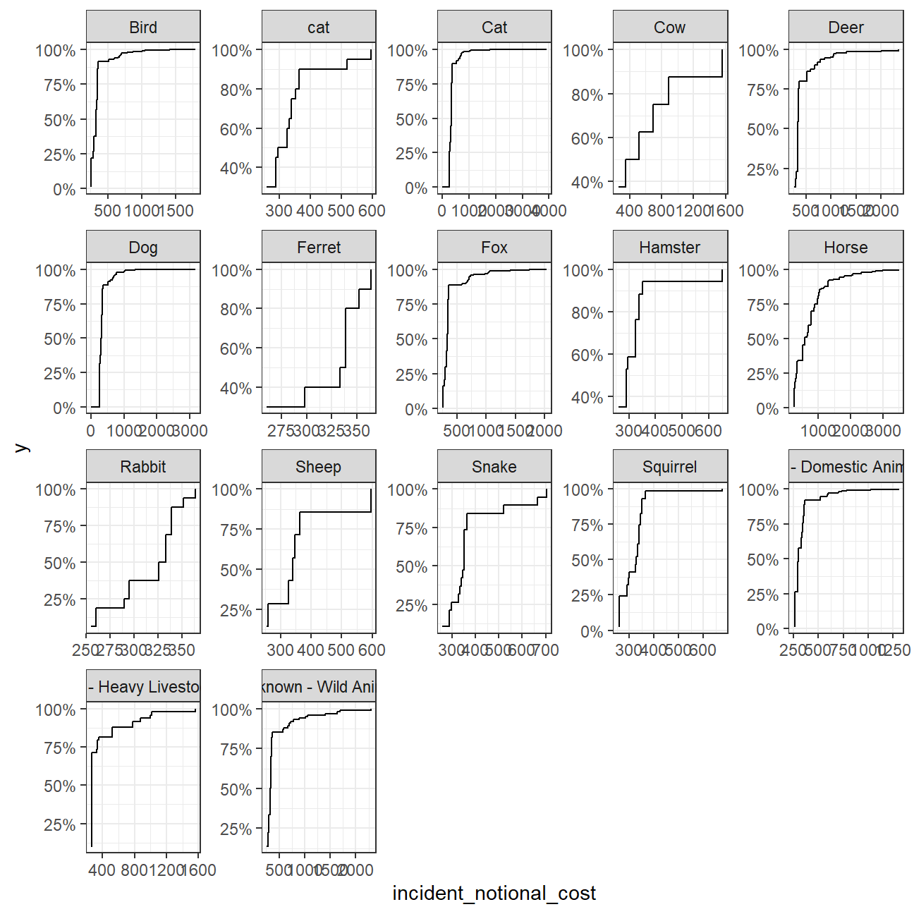
Finally, let us plot a few plots that show the distribution of incident_cost for each animal group.
# base_plot
base_plot <- animal_rescue %>%
  group_by(animal_group_parent) %>%
  filter(n()>6) %>%
  ggplot(aes(x=incident_notional_cost))+
  facet_wrap(~animal_group_parent, scales = "free")+
  theme_bw()

base_plot + geom_histogram()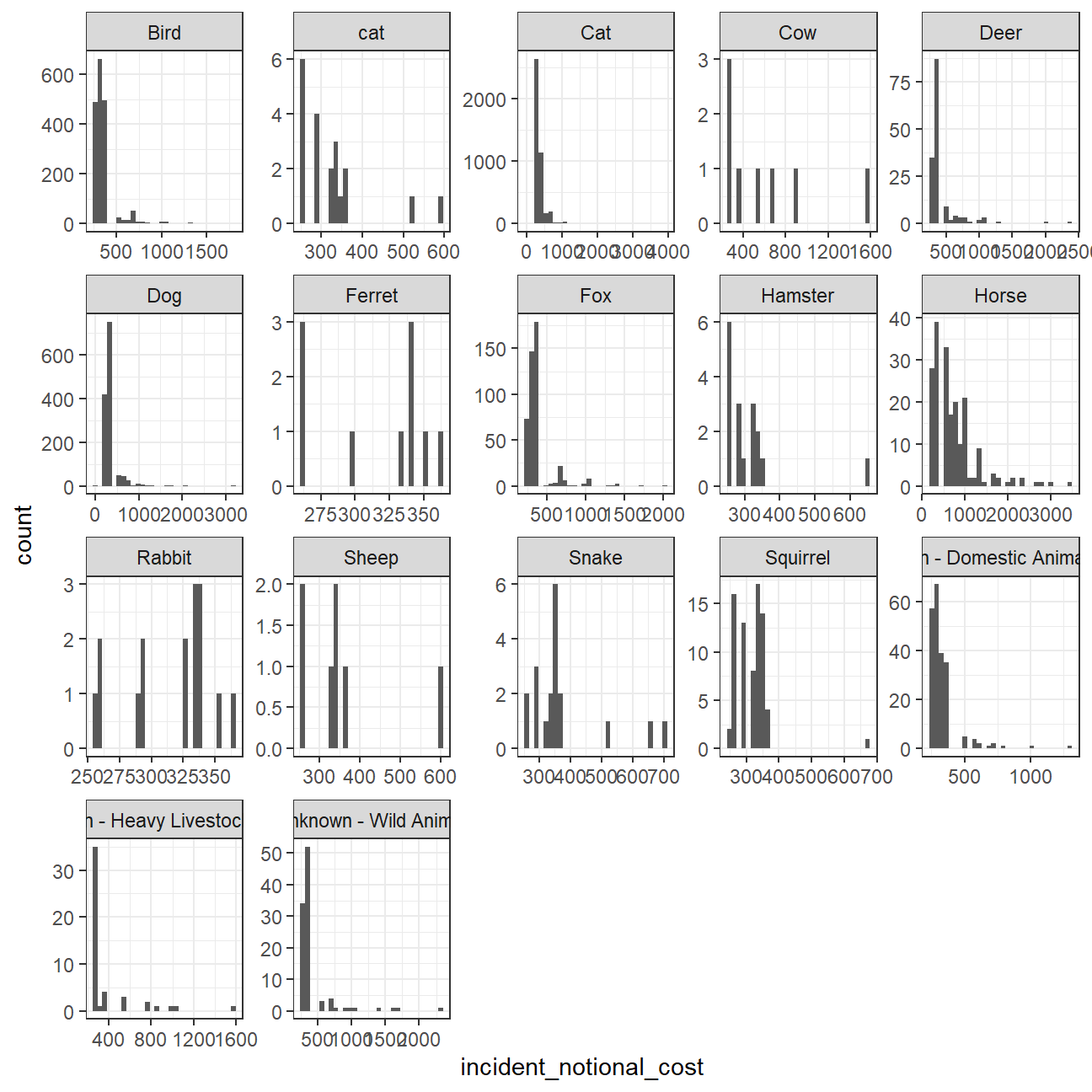
base_plot + geom_density()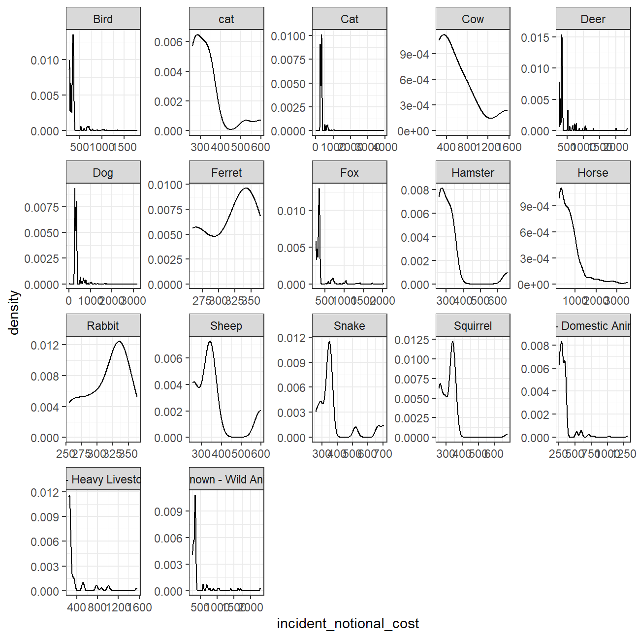
base_plot + geom_boxplot()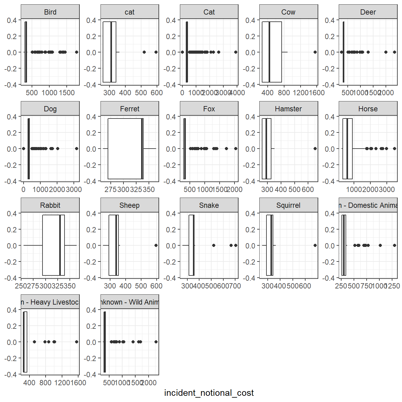
base_plot + stat_ecdf(geom = "step", pad = FALSE) +
  scale_y_continuous(labels = scales::percent)